• Activation Functions
  • Sigmoid
    • Advantages: (-inf , inf) » (0 , 1), good for saturating “firing rate” of neuron
    • Disadvantages:
      • Saturated neuron’s gradient is nearly 0: it stops gradient discent process
      • Sigmoid function is not zero-centered: results of activation function is always positive, which occurs the constraint of gradient discent
      • exp() is compute expansive
  • tanh
    • Advantages: similar with sigmoid, and zero-centered
    • Disadvantages: still saturated neuron kills gradients
  • ReLU(Rectified Linear Unit) = max(0, x)
    • Advantages:
      • Does not saturate in positive region
      • computationally efficient
      • converges faster than sigmoid/tanh
      • more plausible in biological sight
    • Disadvantages:
      • not zero-centered(Some people initialize ReLU neuron with slight positive biases to avoid this drawback)
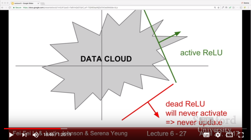
      • gradient vanishes in negative region
  • Leaky ReLU = max(0.1 * x, x)
    • Advantages: Similar with ReLU, and gradients will not die at negative region
    • Similarly we have Parametric Rectifier(PReLU) f(x) = max(ax, x) (a is parameter)
  • ELU(Exponential Linear Unit) = max(a*(e^x - 1), x)
    • Advantages: Similar with ReLU, gradients will not die at negative region, closer to zero mean(centered) function, more robust to noise than Leaky ReLU
    • Disadvantages: Complex computation of exp()
  • Maxout = max(w * x + b, w’ * x + b’)
    • Advantages
      • Has Linear Regime
      • Does not Saturate
      • Generalized version of ReLU / Leaky ReLU
    • Disadvantages: it doubles the number of parameters
  • In Practice: Use ReLU, Try Leaky ReLU / ELU / Maxout, Don’t expect much on tanh, Do not use sigmoid

• Data Preprocessing
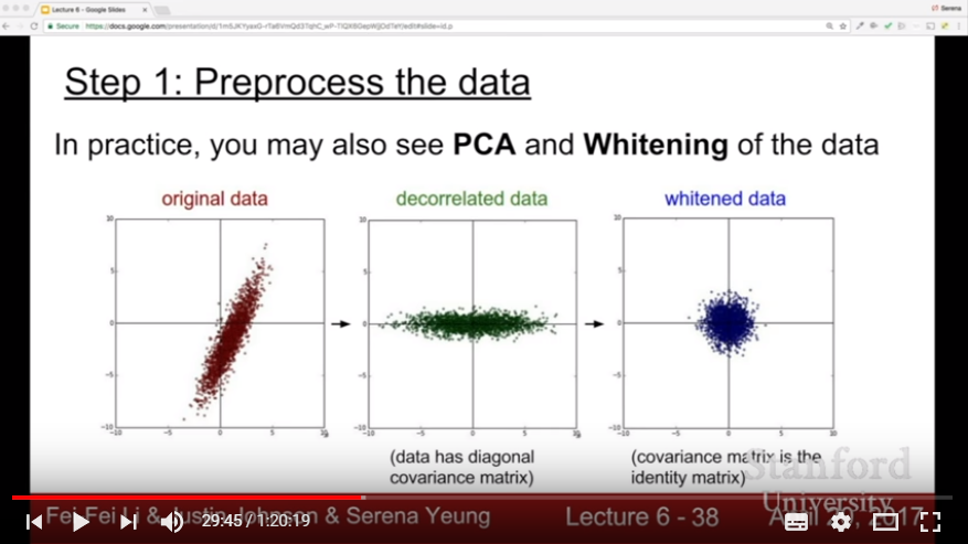
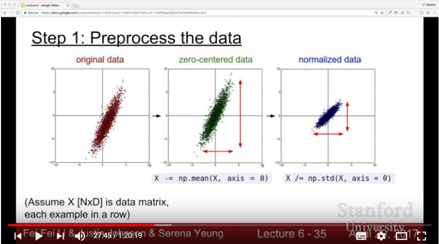
  • There might be a constraint in all-positive or all-negative data: it is good to make data zero-centered
    • For each cases, we do subtract the total mean value or subtract the channel mean value for each channel
  • Another preprocessing might not be needed; since our data is all given pixels, we don’t want to reduce its dimension or scale its description values.

• Weight Initialization
  • If we initialize weight as 0, or other constant value, then every front-propagation and backpropagation computation value would be same for every node; Network would be needless
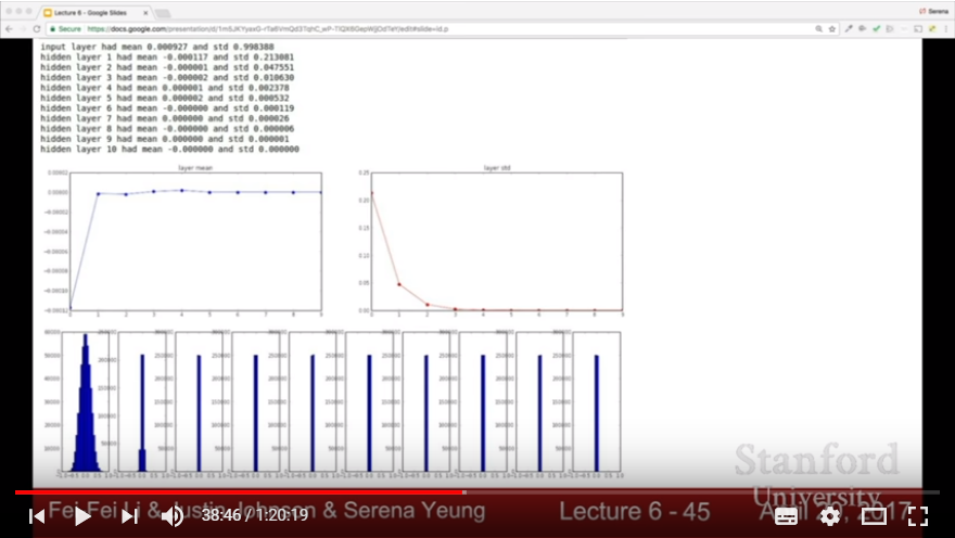
  • If we initialize weight as small random numbers, then as backpropagation between layers proceeds, every gradient goes 0 because of multiplication of small size weight value.
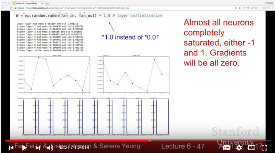
  • If we initialize weight as big random numbers, then neuron nodes would saturate as 1 or -1, gradients would be zero.
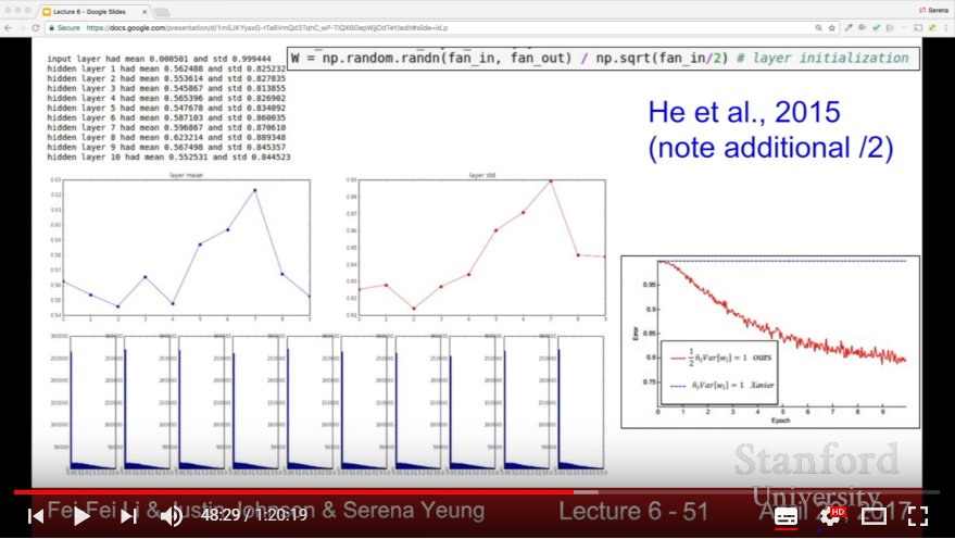
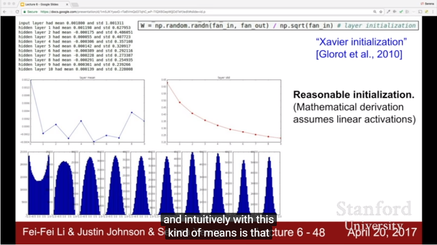
  • reasonable initialization by Xavier initialization {random number in (0,1)} / {root of {# of input node}}
    • In ReLU, we tend to use {root of {# of input node / 2}} instead of {root of {# of input node}}

• Batch Normalization
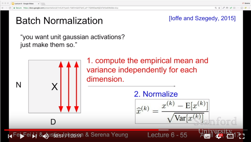
  • Goal: keep the gaussian distribution of activation rate(that is, don’t lead nodes to be dead)
  • Stretagy: Just make it happen! It’s a matter of normalization.
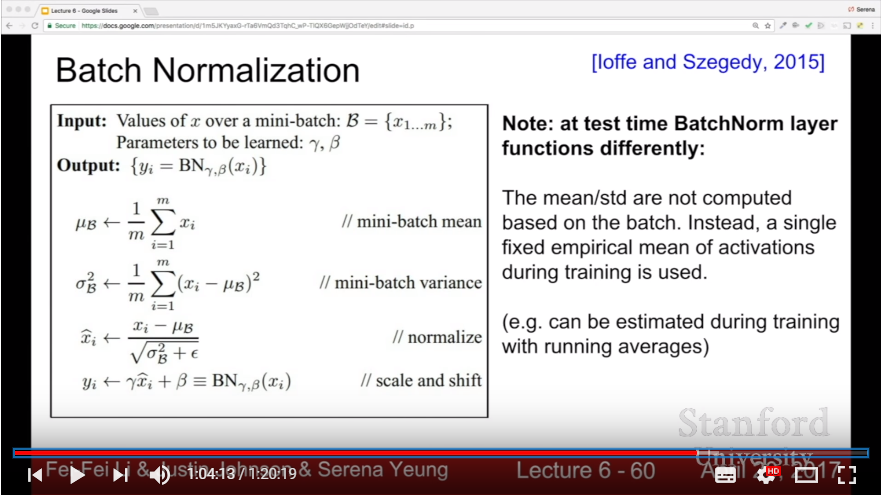
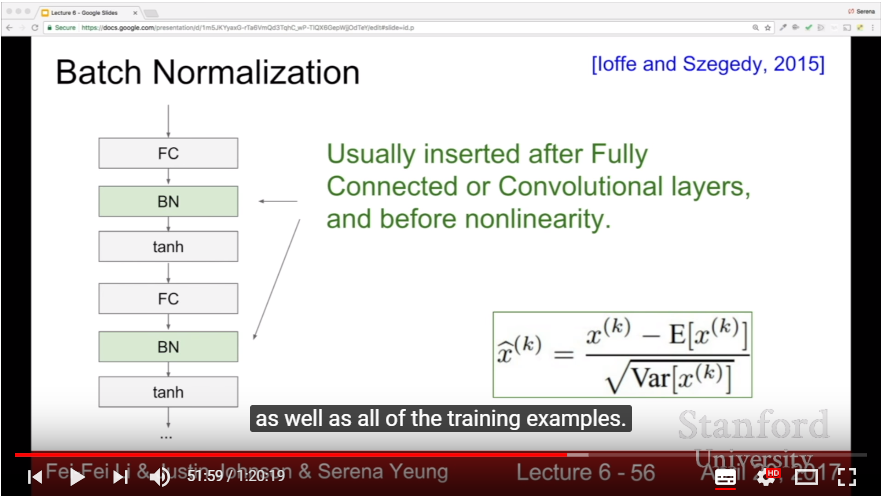
  • Howto: for each dimension(in hidden layer, it might be each node) of mini batch, normalize the values for average and std. It works between FC layer and activation(tanh) function.
  • It gives robustness in range of learning rates/different initialization, and improves gradient flow
  • Practically, instead of using just normalized xhat, we also learn gamma and beta value. It would coordinate the result value while proceeding learning process
  • Practically, instead of solving each batch’s mean/std, we might use single fixed empirical mean/std estimated from first training.

• Babysitting the Learning Process
  • Preprocessing > Choosing architecture > Varient Test > Train Data!
  • Sanity Check: for softmax of 10 classes, it is reasonable to check loss < 2.3 (= 10 * ln(1/10)) Also, we could check the increases of loss when cranking up the regularization.
  • Training Check: for small size of data, check for each epoch, cost goes nearly 0 and accuracy nearly 1. It should be done in small size of data(of course the result will be overfit, but anyway it’s test).
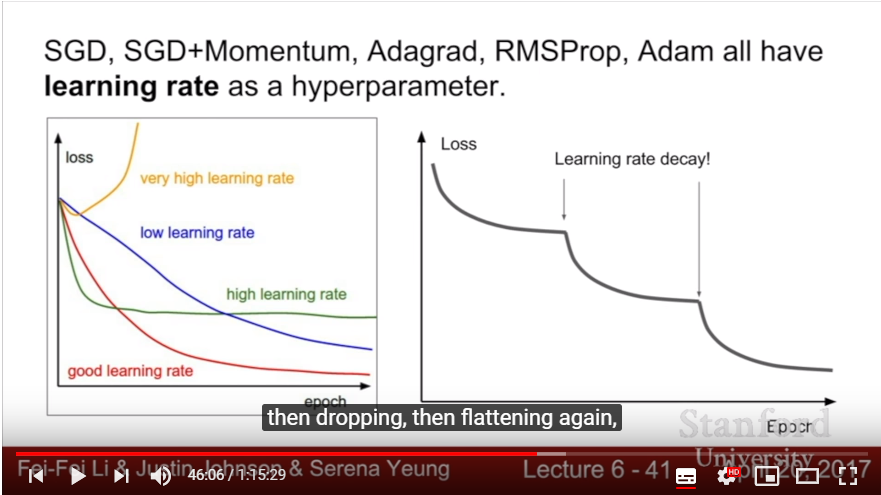
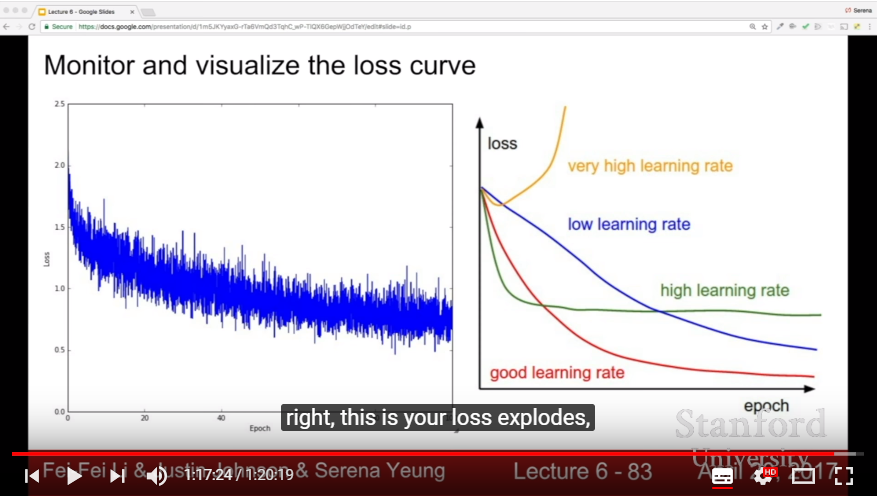
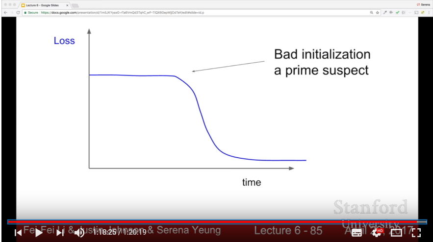
  • Choose reasonable learning rate, otherwise loss would not going down or would explode to inf (1e-3 ~ 1e-5 is sufficient)
• Hyperparameter Optimization
  • Cross Validation Strategy
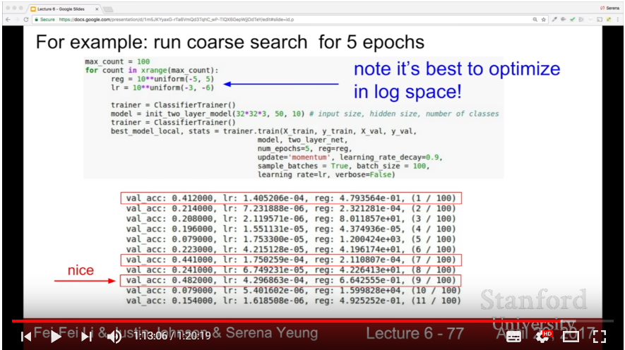
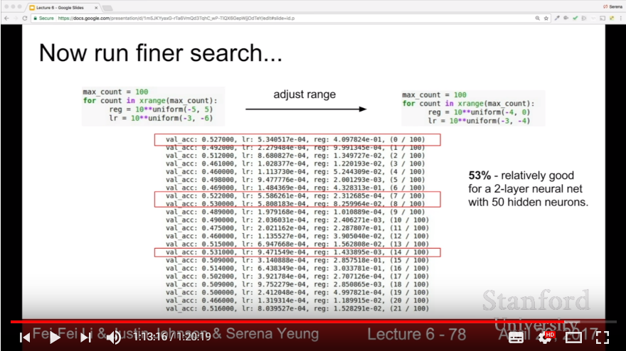
    • For efficiency, first do coarse validation in few epochs. Then do fine validation in valid range of params, more epochs.
    • Do cross validation with log space!
    • Search hyperparameters with Random Search instead of Grid Search: it can find out the signals of distributions of hyperparameters more naturally.
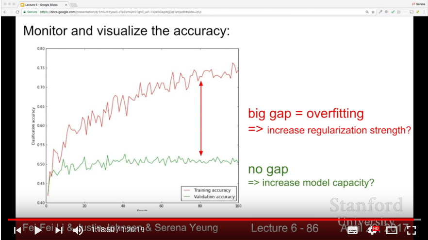
  • Monitering the Hyperparameters with graph, or some indicator(ex: {gap between training acc and validation acc}, {weight updates}/{weight magnitudes})

• Optimization Stretagy
  • Problem:
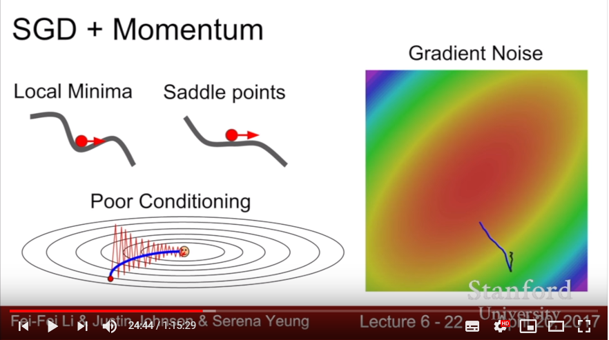
    • SGD might be stuck in local minima or saddle point(especially, there will likely more saddle point than local minima in high dimension)
    • SGD might be noisey: since it calculates gradient from minibatch of data.
  • Solution:
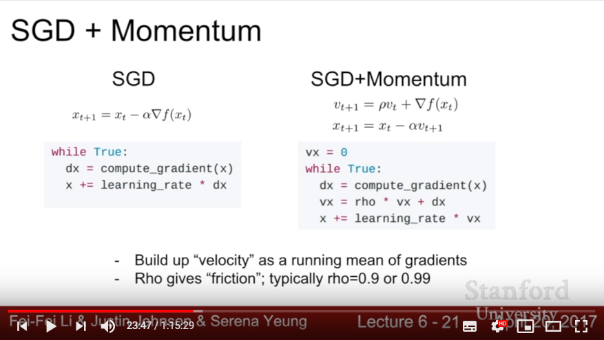
    • add Momentum at SGD.
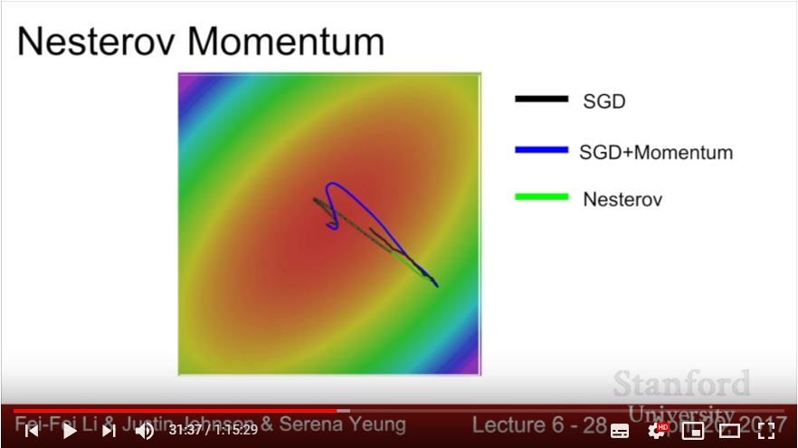
    • there also exists another way of calculating momentum: in Nesterov Momentum, we add small piece of velocity when calculating gradient of given x. In that way, velocity works as correction term of gradient; it helps shortening the scale of overfitting.
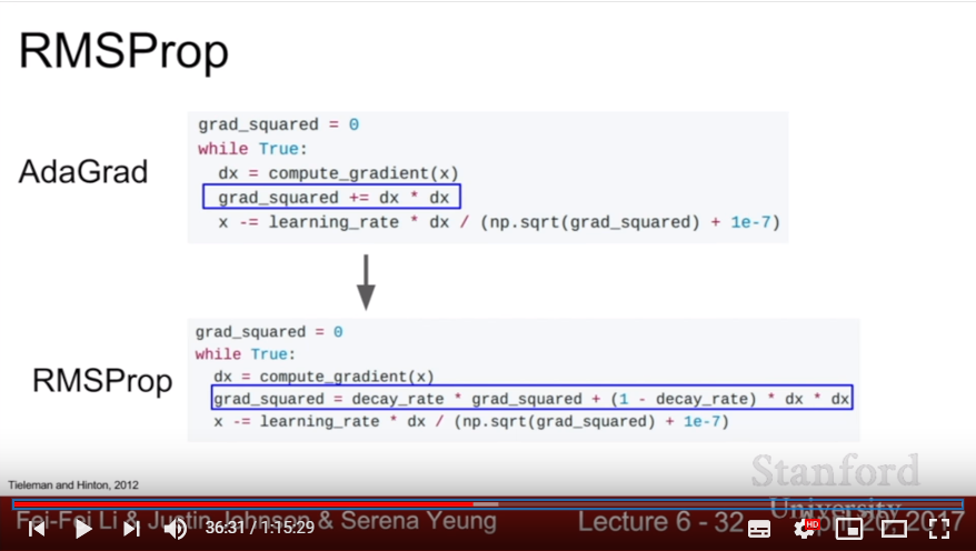
    • AdaGrad: Compute the sum of gradient-squared. While subtracting gradient, divide this gradient-squared value so that the updates goes smaller each time.
      • It scales the gradient (which is too huge in some dim, and too small in another) reasonably, and can also reduces updates
      • But in non-convex data, this would not reach global minima because update is just shortened to reach minima, not global one. We usually not use AdaGrad in real cases.
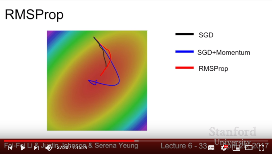
    • RMSProp: use the momentum method in gradient-squared; take decay_rate(about 0.9) to gradually modify gradient-squared
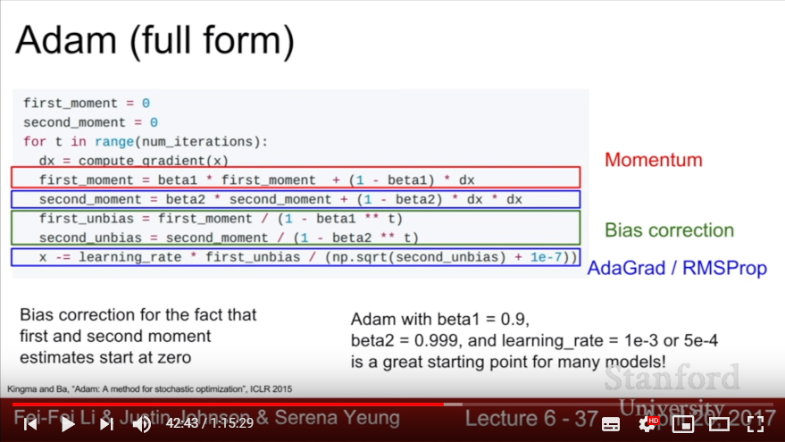
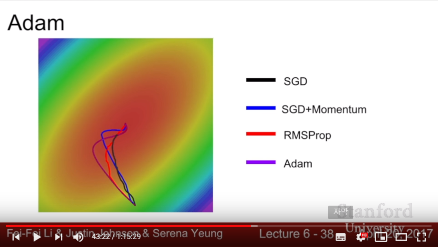
    • Adam: use Momentum method and concept of AdaGrad(RMSProp) that use gradient-squard!
      • But as we set the initial size of second_moment 0, (and gradually increase second_moment with beta2 nearly 0.9) it would make a big update in initial gradient update.
      • To correct this big changes in first state, we add bias correction term and divide (1 - {beta} ^ {current time step}). This would scale up the first moment and second moment in initial state, then corrects the big update.
      • Initial size of beta1 = 0.9, beta2 = 0.999, learning rate = 1e-3 would be great for almost every learning problem!
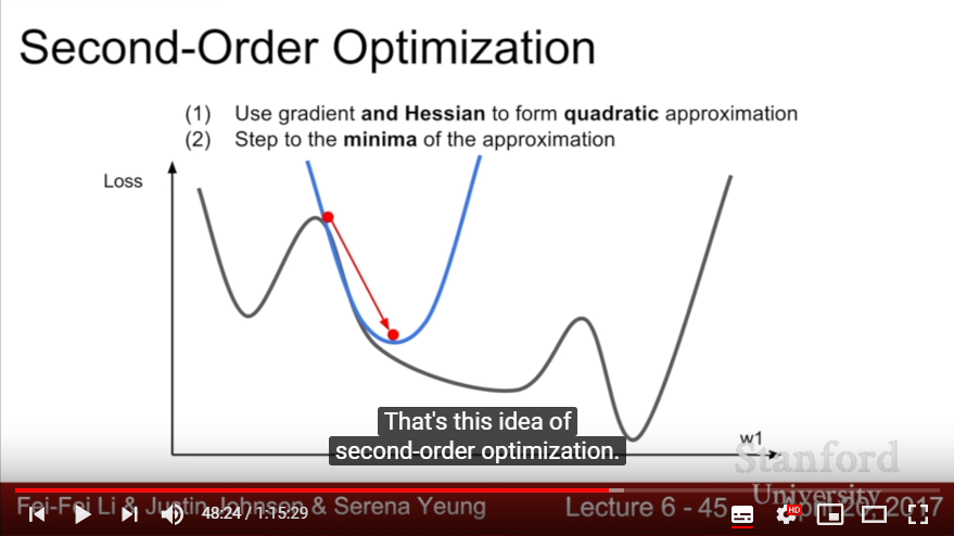
  • Second-Order Optimization
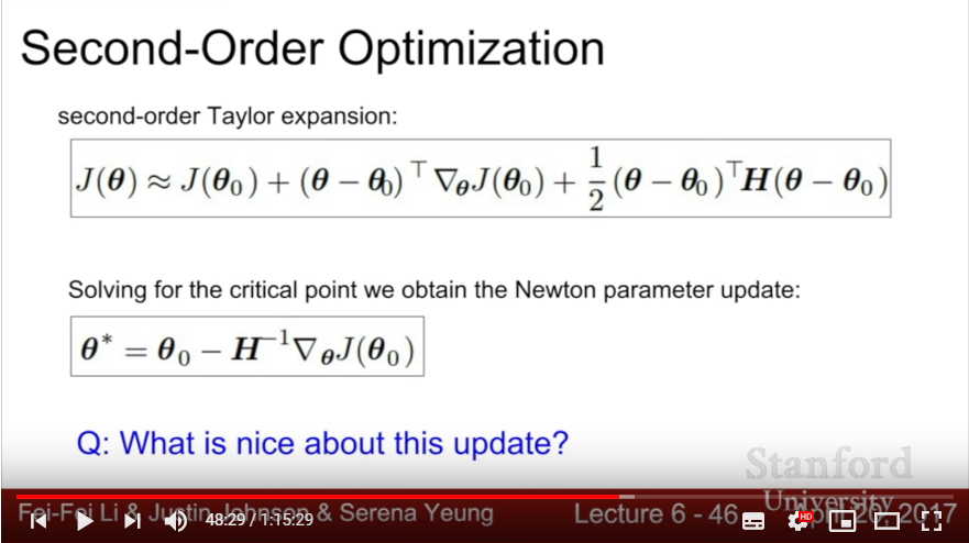
    • SGD is first-order optimization method in Taylor-Expression point of view
    • Instead of using SGD, Use Quadratic Approximation and set the next step to ‘minima of quadratic function’
      • Also called ‘Newton Step’
    • Use gradient + Hessian
      • Hessian: Matrix of second derivatives
    • Since we step to minima of quad func, we don’t need any learning rate(but just in the vanilla Newton Step)!
    • But Since Hessian has O(N^2) & Inverting Hessian takes O(N^3), it is totally unefficient. (it might even not be able to save in memory)
      • We use low-level approximation method of Hessian Matrix, Quasi-Newton Method or L-BFGS(Limited memory BFGS), to overcome it.
      • L-BFGS works well in full batch learning, but it doesn’t work well with stochastic method. Also, it might not work with non-convex case. (It is an active area of research)
      • In practice, Adam is good choice in most cases, and if we use full batch updates (and it is convex, that is there are no noise sources), trying out L-BFGS might be a good choice.

• Learning Rate Choosing Stretagy
  • Step decay: Decaying learning rate after specific iterations proceeded. (Exponential decay, 1/t decay)
  • Usually used with Momentum(which occurs overfitting while epoch goes), but usually not used in Adam.
  • In practice, usually first learn without decay; then determine that this problem would need Decaying stretagy,

• Regularization and Method of Reducing Overfitting
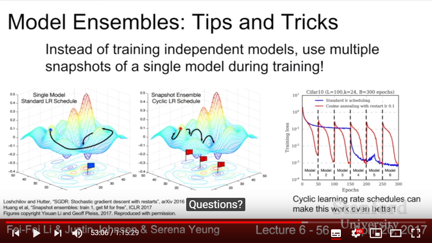
  • Model Ensembles: Train multiple modles and time average the results at test case.
    • This gives about 2 percent-improvement, and it would be consistent.
    • Instead of making multiple model, give a ayclic learning rate and take snapshot of converged result is also a useful method!
  • Polyak Averaging: Instead of using parmeter vector, use moving average of parameter vector(but not common in practice)
  • Regularizaion Method
    • L2 Regularization doesn’t make sense in NN
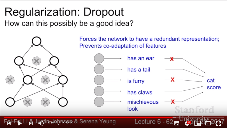
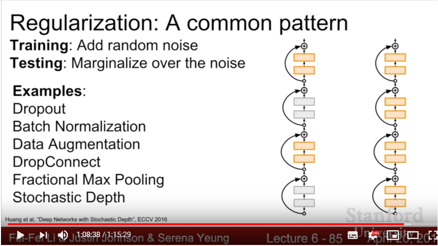
    • Dropout: In each forward pass, randomly set some neurons to zero
      • Usually take probability of dropping neuron as 0.5(hyperparameter)
      • Avoid the co-adaptance of each features
      • Or, it can be interpreted as ‘training a large ensemble of subnetworks in one network’
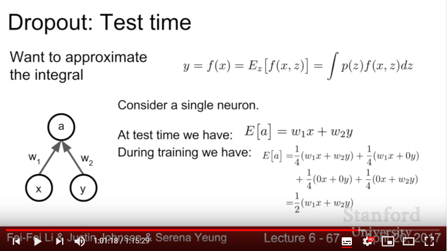
      • Eliminate the stochasticity of random dropout mask in test session, then we should average the result of each nodes instead of only summing it. (That is, multiply the dropout prob in the test time)
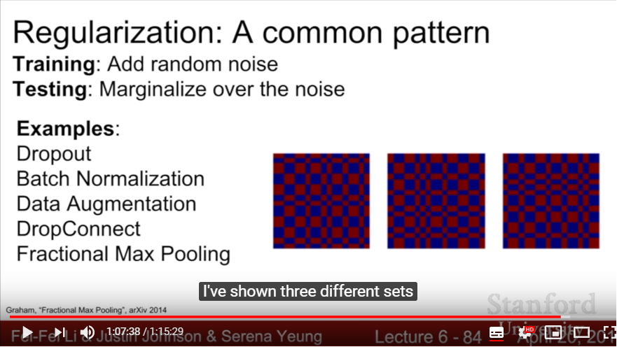
    • Batch Normalization do has some similar work of Dropout: While in training, normalize random minibatches with the stats of minibatchs, then use fixed stats when testing. Then the stochasticity of each single data point would be somewhat normalized.
      • But Dropout has some advantage that we could choose the parameter prob of dropout.
    • Data Augmentation
      • Transform the data in some way(ex: flips, crops, translations, rotation, stretchings, shearings, color jittering in contrast and brightness). We use random combinations of these methods.
    • DropConnect: zero out some values of weight matrix with specific prob, instead of nodes.
    • Fractional Max Pooling: Randomly choose where we do max pooling 2 * 2 pixels.
    • Stochastic Depth: Randomly drop ‘layers’ during the training time, then use whole layers in test.
    • In practice, usually batch normalization is enough for regularization. If overfitting happens even if we use batch normalization, consider using Dropout.
  • Transfer Learning
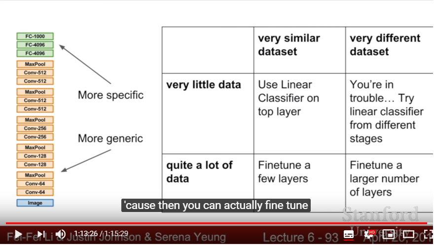
    • Problem: Whenever we use large & deep CNN methods, it usually happens to overfit because of our small dataset
    • When-to-use: we want to train small classes(ex: 10 dog breeds) with small dataset
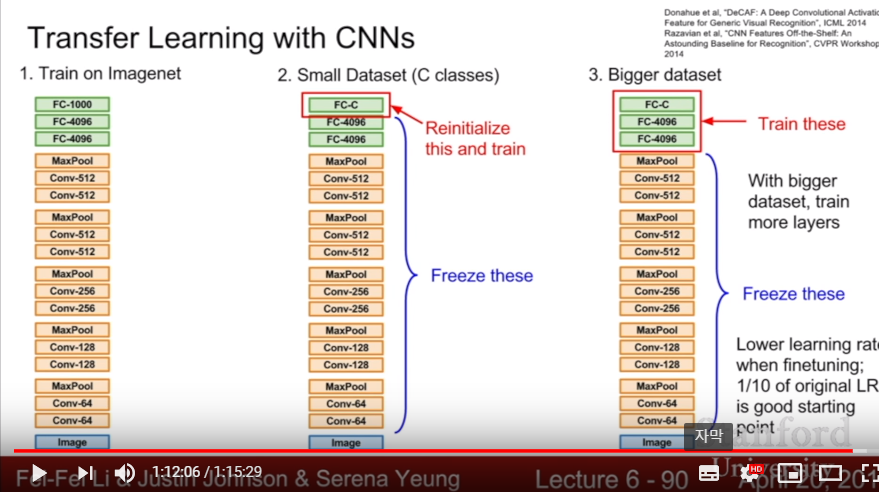
    • After we train versatile, HUGE dataset(like Imagenet) for our large CNN Model(with 1000 classes, that is, 4096 * 1000), we reinitialize the last weight matrix and resize it with 4096 * 10. Then re-train!
    • The model which is good for classifying 1000 classes will be also good at classifying 10 classes. What we need to do is only re-training last layer.
    • For more bigger dataset, train FCNN layers, with freezing Conv layers.
    • Since this is re-training, we should lower learning rate with 1/10 of original lr.
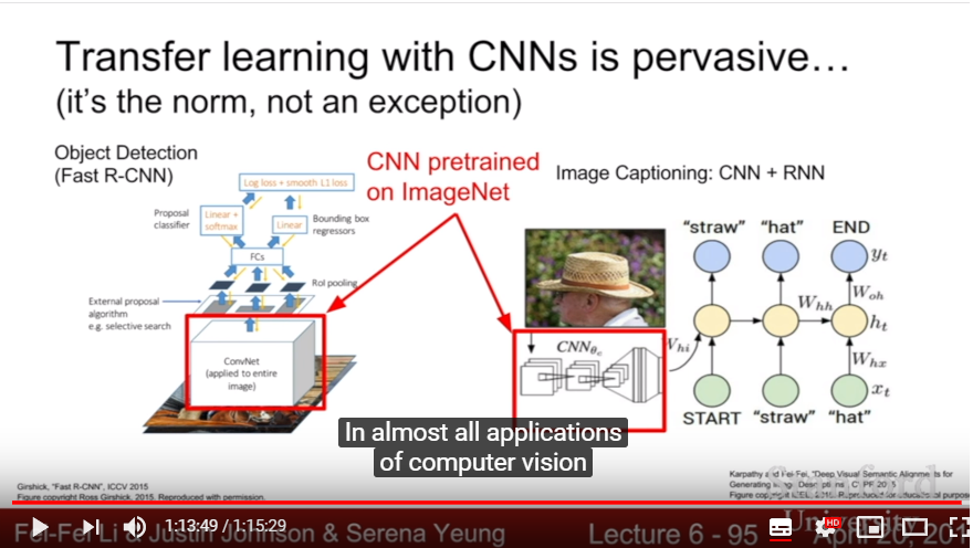
    • SUPER pervasive! It’s a norm, not an exception
    • DL frameworks provide a ‘Model Zoo’ of pretrained models, so just download it and use it in your own task